k-Nearest Neighbors (kNN)
The basic idea behind the k-Nearest Neighbors algorithm is that similar data points will have similar labels. kNN looks at the k most similar training data points to a testing data point. The algorithm then combines the labels of those training data to determine the testing data point's label.
For our k-Nearest Neighbors classifier, we used Euclidean distance as the distance measure, which is calculated as shown below. There are many other possible distance measures including Scaled Euclidean and L1-norm.

Calculation of Euclidean Distance
After determining the k-nearest neighbors, the algorithm combines the neighbors' labels to determine the label of the testing data point. For our implementation of k-Nearest Neighbors, we combined the labels used a simple majority vote. Other possibilities include a distance-weighted vote, in which labels of data points that are closest to the testing point have more of a vote for the testing point's label.
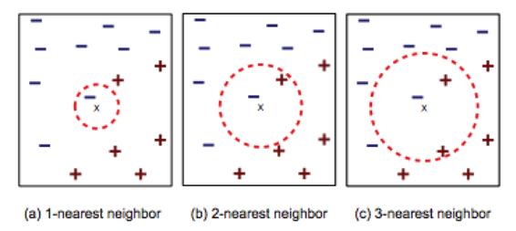
k-Nearest Neighbors algorithm for (a) k =1, (b) k = 2, (c) k = 3.
Image Credit: MIT Opencourseware
Decision Tree
The decision tree algorithm aims to build a tree structure according to a set of rules from the training dataset, which can be used to classify unlabeled data. In this study, we used the well-known iterative Dichotomiser 3 (ID3) algorithm invented by Ross Quinlan to generate the decision tree.
This algorithm builds the decision tree based on entropy and the information gain. Entropy measures the impurity of an arbitrary collection of samples while the information gain calculates the reduction in entropy by partitioning the sample according to a certain attribute [cite]. Given a dataset D with categories cj, entropy are calculated by the following equation:
This algorithm builds the decision tree based on entropy and the information gain. Entropy measures the impurity of an arbitrary collection of samples while the information gain calculates the reduction in entropy by partitioning the sample according to a certain attribute [cite]. Given a dataset D with categories cj, entropy are calculated by the following equation:
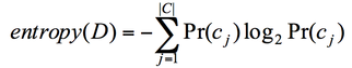
Entropy and information gain is related by the following equation, where entropyAi (D) is the expected entropy is attribute Ai is used to partition the data.
The algorithm was implemented according to the following steps:
1) Entropy of every feature at every value in the training dataset was calculated.
2) The feature F and value V with the minimum entropy was chosen. If more than one pair have the minimum entropy, arbitrarily chose one.
3) The dataset was split into left and right subtrees at {F, V} pair.
4) Repeat the steps 1-3 on the subtrees until all the resulting dataset is pure, i.e., only contains one category. The pure data are contained in the leaf node.
By splitting dataset according to minimum entropy, the resulting dataset has the maximum information gain and thus impurity of the dataset is minimized. After the tree is built from the training dataset, testing data point can be fed into the tree. The testing data will go through the tree according to the predefined rules until reaching a leaf node. The label in the leaf node is then assigned to the testing data.
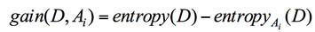
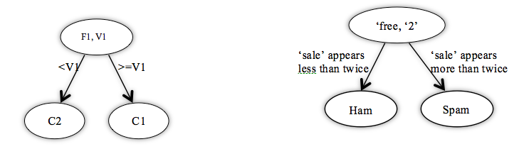
The conceptual tree and the tree example with spam filter. F refers the features, or words in the case of spam filter. V refers the values, or word frequencies in this case. C represents the labels, which are spam/ham for spam filter.
Pruned Decision Tree
The ID3 tree algorithms introduced above requires all leaf nodes to contain pure data. Thus, the resulting tree can overfit training data. A pruned tree can solve this problem and improve the classification accuracy and computation efficiency.
Suppose the ID3 tree without pruning is T and the classification accuracy by T as TAccuracy. Pruning iteratively deletes subtree of T at the bottom to form a new tree and reclassify the testing data using the new tree. If the accuracy increases from TAccuracy, then the pruned tree will replace T. The resulting pruned tree has less nodes, smaller depth and higher classification accuracy.
Suppose the ID3 tree without pruning is T and the classification accuracy by T as TAccuracy. Pruning iteratively deletes subtree of T at the bottom to form a new tree and reclassify the testing data using the new tree. If the accuracy increases from TAccuracy, then the pruned tree will replace T. The resulting pruned tree has less nodes, smaller depth and higher classification accuracy.
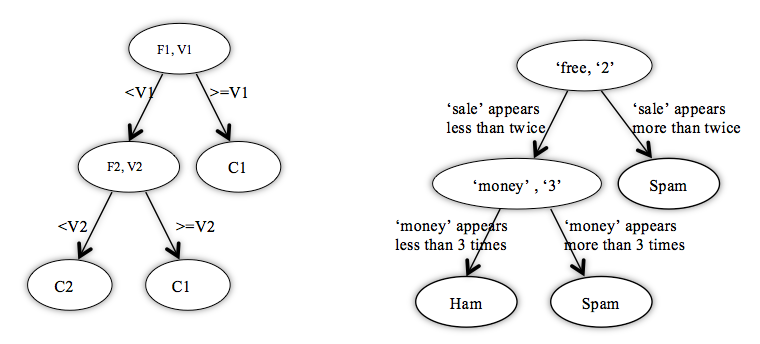
The conceptual pruned tree and the pruned tree example with spam filter. The left subtree at the bottom of unpruned tree was deleted.
Naive Bayesian
The Naive Bayesian classifier takes its roots in the famous Bayes Theorem:

Bayes Theorem essentially describes how much we should adjust the probability that our hypothesis (H) will occur, given some new evidence (e).
For our project, we want to determine the probability that an email is spam, given the evidence of the email's features (F1,F2,...Fn). These features F1, F2,...Fn are just a boolean value (0 or 1) describing whether or not the stem 1 through n appears in the email. Then, we compare P(Spam|F1,F2,...Fn) to P(Ham|F1,F2,...Fn) and determine which is more likely. Spam and Ham are considered the classes, which are represented in the equations below as "C".
For our project, we want to determine the probability that an email is spam, given the evidence of the email's features (F1,F2,...Fn). These features F1, F2,...Fn are just a boolean value (0 or 1) describing whether or not the stem 1 through n appears in the email. Then, we compare P(Spam|F1,F2,...Fn) to P(Ham|F1,F2,...Fn) and determine which is more likely. Spam and Ham are considered the classes, which are represented in the equations below as "C".

Equation used to determine the class (either C = Spam or C = Ham) given a set the email's features.
Note that when we are comparing P(Spam|F1,F2,...Fn) to P(Ham|F1,F2,...Fn), the denominators are the same. Thus, we can simplify the comparison by noting that:

Calculating P(F1,F2,...Fn|C) can become tedious. Thus, the Naive Bayesian classifier makes an assumption that drastically simplifies the calculations. The assumption is that the probabilities of F1, F2, ..Fn occurring are all independent of each other. While this assumption is not true (as some words are more likely to appear together), the classifier still performs very well given this assumption. Now, to determine whether an email is spam or ham, we just select the class (C = spam or C = ham) that maximizes the following equation:

Decision criterion for Naive Bayes classifier
Logistic Regression
Logistic Regression is another way to determine a class label, depending on the features. Logistic regression takes features that can be continuous (for example, the count of words in an email) and translate them to discrete values (spam or not spam). A logistic regression classifier works in the following way:
1. Fit a linear model to the feature space determined by the training data. This requires finding the best parameters to fit the training data
1. Fit a linear model to the feature space determined by the training data. This requires finding the best parameters to fit the training data
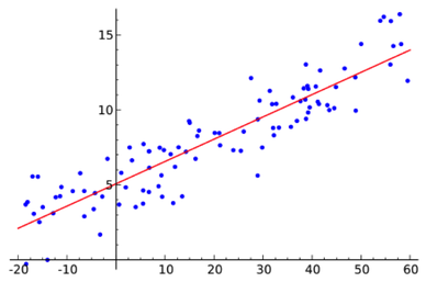
An example of a linear model fit to the feature space.
Image credit: http://en.wikipedia.org/wiki/File:Linear_regression.svg
|
The model is an n-dimensional vector given by the equation below:

|
2. Using the parameters found in step 1, determine the z value for a testing point.
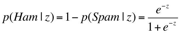
3. Map this z value of the testing point to the range 0 to 1 using the logistic function. This value is one way of determining the probability that these features are associated with a spam email.
3. Map this z value of the testing point to the range 0 to 1 using the logistic function. This value is one way of determining the probability that these features are associated with a spam email.
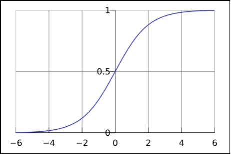
The logistic function.
Image credit: http://en.wikipedia.org/wiki/File:Logistic-curve.svg
|
As shown on the left, the logistic function helps us translate a continuous input (the word counts) to a discrete value (0 or 1, or equivalently, ham or spam.)

|
